1.3 Reading a Datasheet

After this section you can: read sensitivity, range, frequency limits against mounted resonance, transverse and base-strain sensitivity, temperature effects and mass, and say which one limits this test.

A datasheet is a page of numbers for a model, and most of them never matter on a given test. One or two of them do, and which ones depends on the test. This section goes down the page in the order a test engineer reads it, and ends with how to tell which line limits the test in hand.

Sensitivity comes first, with a tolerance beside it. The datasheet's figure is the nominal for the model; the certificate's figure is what this serial number measured at the reference frequency on the day it was calibrated, and that is the number entered for the channel (1.7). Two sensors of the same model can differ by most of the tolerance, so a sensitivity belongs to a serial number, never to a model. A channel table that carries a model's nominal sensitivity, or the last sensor's, is wrong by however far the two differ, and nothing on the screen will show it (1.1).

Range comes next, and range is where the sensor is most often wrong for the test. The trap is to compare the range with the profile. The sensor does not see the profile. It sees the response at the point it is mounted, and the response at a resonance is many times the input. A sine input of 2 g on a resonance with a Q of 25 (the ratio of the response at resonance to the input, which Chapter 6 takes in full) is a response of 50 g, which is the whole range of a 100 mV/g IEPE sensor. A random response channel reading 15 grms (its overall rms level, in g) has peaks of three times that, 45 g, many times in a minute and higher ones now and then, because a random signal's peaks run to three standard deviations and beyond (Chapter 7). A shock response rings at the article's modes at more than the pulse's peak. And all of these are in band. The sensor also sees what is out of band: a fastener chattering, an article rattling in its mount, metal striking metal, all of which put energy into the sensor's own resonance, far above the test band. An IEPE sensor's built-in amplifier saturates on that energy just as it would on in-band energy, and the filters downstream remove the evidence. One sensor manufacturer's note on accelerometer faults (PCB Piezotronics TN-30) says plainly that a saturated sensor can go unnoticed if only the frequency-domain data is viewed. 1.8 shows what it looks like. Setting the input range on the controller is 2.3's subject. The sensor's own range is this chapter's, and it is the one that cannot be fixed afterwards: once the amplifier inside the case has saturated, nothing downstream can recover the signal. For shock, Method 516.8 asks in paragraph 4.4 for amplitude linearity within 10 percent over the range the measurement uses.

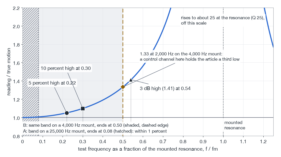
Then the frequency limits. The datasheet gives a frequency range, usually stated as the band within plus or minus 5 percent or within 3 dB, and a resonant frequency. Both were measured with the sensor stud-mounted on a stiff calibration fixture. On the test, the number that counts is the mounted resonance, the resonance of this sensor on this mount on this surface, and it is never higher than the datasheet's and often a good deal lower (1.4). Below its mounted resonance the sensor reads high by an amount that grows as the test frequency climbs toward it. The Bruel and Kjaer handbook on piezoelectric accelerometers (Serridge and Licht) gives, for one of its general-purpose sensors, a reading 5 percent high at about 0.22 of the mounted resonance, 10 percent high at about 0.30, and 3 dB high at about 0.54. Those are that handbook's figures for its sensor. They are also what a single, lightly damped resonance gives, which lets the same arithmetic be done for any sensor (the author's arithmetic, not the handbook's):

where:

• $\text{reading}$: the acceleration the sensor reports, g
• $\text{true}$: the acceleration at the mounting surface, g
• $f$: test frequency, Hz
• $f_m$: mounted resonance of the sensor, Hz

At $f/f_m = 0.22$ the formula gives 1.05, at 0.30 it gives 1.10, and at 0.54 it gives 1.41, which is 3 dB.

That arithmetic carries a decision. Method 514.8, in paragraph 4.2.3, asks for an accelerometer flat within plus or minus 5 percent across the frequency range of interest, and Method 516.8, in paragraph 4.4, asks the same for shock, relaxed to 1 dB for high-range sensors with low output. By the arithmetic, a 5 percent limit puts the top of the test band at no more than about 0.22 of the mounted resonance. A random test to 2,000 Hz then needs a mounted resonance above about 9,000 Hz. A sensor whose datasheet resonance is, say, 25,000 Hz has that with room to spare on a stud. The same sensor on a mount that has brought its resonance down to 4,000 Hz, whatever the reason, reads a third high at 2,000 Hz, and a control channel on it holds the article a third low.

a. The reading across the fraction of mounted resonance

One lightly damped resonance (Q 25). Circle, square and triangle: 5 percent, 10 percent and 3 dB high. The band of a 2,000 Hz random test on a 25,000 Hz mount (hatched, A) and on a mount gone soft to 4,000 Hz (shaded, B).

b. Inset: the resonance excited from far above the band

The same sensor on its 25,000 Hz mount, with no filter (solid) and with a built-in two-pole low-pass at 8,000 Hz (dashed). In band they agree; at the resonance the filter cuts the peak about tenfold.

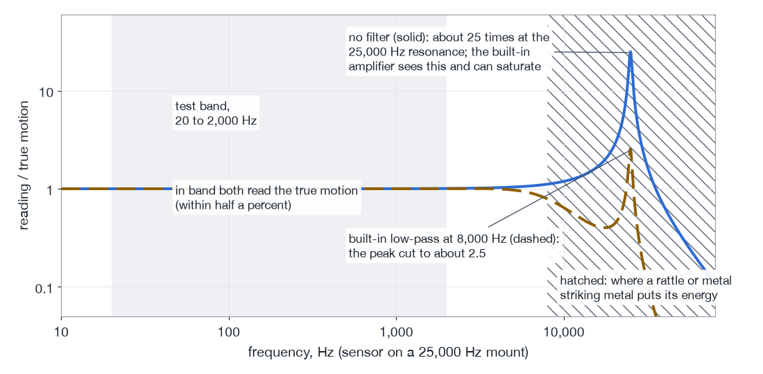
Synthetic, the author's model; every value assumed and stated in the notes. The marks are the single-resonance arithmetic of the text.

The low end of the frequency range is set by the time constant (1.2) on a piezoelectric sensor and is zero on a piezoresistive or capacitive one. The datasheet gives it as a frequency, a time constant or both, and 1.5 turns it into the error at the bottom of a long-stroke sine.

Transverse sensitivity is the response to motion across the measuring axis, as a percentage of the main sensitivity: 5 percent or less for 514.8, 7 percent or less for 516.8. It is usually small, and it stops being small exactly where the cross-axis motion is large. Cube fixtures (a hollow block bolted to the table with the article on one of its side faces, so that the article can be driven in a lateral axis on a vertical shaker) are the case: at their first resonance their article faces move across the test axis by more than they move along it, in the author's models by about half again as much, one and a half times. A sensor with 5 percent transverse sensitivity on such a face, with the cross motion one and a half times the in-axis motion, carries an error of up to one and a half times 5 percent, about 8 percent, in its in-axis reading at that frequency (the author's arithmetic), and how much of that reaches the reading depends on which way the cross motion lines up with the sensor's most sensitive transverse direction. The datasheet gives the maximum, not the direction.

Base-strain sensitivity is the output from bending of the surface under the sensor, given as an equivalent acceleration per microstrain. Method 514.8 asks that it be evaluated, and the evaluation is a judgment about the surface. On a thick fixture block it does not matter. On a fixture plate with a bending mode in band, or on an article's thin panel, it can matter more than any other line on the page, and a shear design keeps it small (1.2).

Temperature shows up twice. The first is the operating limit, the hottest and coldest the sensor will stand, which for an IEPE sensor is set by its electronics and varies by model. The second is how the sensitivity changes with temperature, usually as a curve. Method 514.8 asks in paragraph 4.2.3 for a deviation no more than plus or minus 5 percent at the test temperature relative to the calibration temperature, so on a chamber test the curve is read at the chamber's extremes, not at room temperature. A sensor that passes at both ends of the chamber and fails in the middle of a transition is the compression design's thermal drift, 1.2's point.

Mass is last on most datasheets and first on a light article. A sensor bolted to a structure is part of the structure, and on a light one it pulls the resonances down. The author's practice is to keep a sensor below one-tenth of the structure's local mass at the point it is mounted: the mass that moves with that point in the structure's mode there, which for a thin lid or a bracket is a small part of the whole. (This is not the effective mass of 6.5, which is the share of an article's mass that a mode moves as seen from its mounting interface.) That is a practice, not a standard, and the reason for one-tenth is the same square-root rule that moves the armature's resonance under a fixture: a resonance falls as one over the square root of the mass it carries, so adding a tenth to the mass pulls it down by about 5 percent, small enough that the structure's modes are still the structure's. On a fixture it never matters. On a small bracket, a circuit board or a thin cover it can decide which sensor goes on, or whether a non-contact instrument has to be used instead.

Down the page, then, every line is a question about the test, and on most tests one of them answers no. Take a small electronics box in a hot chamber, random to 2,000 Hz, with a response channel on its thin lid. The range question is the lid's response at its own resonance. The frequency question is how the sensor can be mounted on a painted lid the owner will not let anyone drill. The temperature question is the chamber against the IEPE datasheet. The mass question is the lid itself, which may weigh little more than the sensors the analyst wants on it. Any one of the four can rule out the sensor in the drawer. The point of reading the page is to find out which one before the sensor is on, not after the data has come back strange.

Worked through, with every number assumed for the illustration (the arithmetic is the author's), the case runs like this. The analyst predicts 18 grms at the lid's center at full level, with the lid's first mode inside the band. At a peak factor of five for headroom that is 90 g, so the 100 mV/g sensor in the drawer, which reaches its 5 V at 50 g, is out on range before anything else is asked; a 10 mV/g sensor reaches 500 g. The lid weighs 3 oz, and the share of it that moves with its center in that mode is taken as about a quarter, 0.75 oz. A general-purpose sensor on a cementing stud weighs about 0.4 oz, half of that; a miniature 10 mV/g sensor of 0.04 oz glued straight to the lid is about a twentieth, which pulls the lid's mode down by under 3 percent. The owner agrees before the article arrives to a cleaned spot the size of the sensor's base, because paint under the base is a soft spring, and the glue is a stiff epoxy rated past the chamber's top temperature of 160 F (71 C), cured overnight. A tap on the mounted sensor (1.4) puts its mounted resonance at 14,000 Hz, so 2,000 Hz is 0.14 of it, inside the 0.22, and the mount is good to about 3,100 Hz. The sensor's datasheet allows 250 F, and its sensitivity curve, read at 160 F, stays inside 5 percent of its room-temperature calibration. Its 60 ft run at 30 pF per foot carries about 53,000 Hz at 4 mA even at the sensor's full 5 V, and its discharge time constant of 0.2 second puts the low corner at 0.8 Hz, far below the band's 20 Hz. The channel-table row (2.4) then reads:

• Name and location: lid, center, Z; the center of the top lid, with the drawing reference and a photograph.
• Axis and sign: Z, positive out of the lid.
• Sensor: the miniature model and its serial; 10.2 mV/g from its certificate, entered at 10.2 with the conditioner at unity gain, 4 mA.
• Coupling and low-frequency limit: AC; 5 percent low at about 2.4 Hz, three times the corner.
• Range: 500 g usable, the sensor's, smaller than the input's at its 10 V range; 90 g predicted peak.
• Mount and its limit: epoxy on bare metal, cured overnight; mounted resonance 14,000 Hz by tap; trusted to 3,100 Hz.
• Temperature: sensor 250 F and adhesive rated past 160 F; sensitivity within 5 percent at 160 F.
• Role: response, stored on the controller and on the independent recorder.