1.8 When a Sensor Lies
about 15 minutes · 4 figures, 2 interactive · quiz of 5 · Slides
After this section you can: recognize bias faults, saturation and its exponential decay, zero shift, ground-loop hum, cable noise, sensor resonance, temperature effects and a loosening mount in the time history and the spectrum.
When a channel shows something strange, there are two candidates, the article and the chain, and the chain is far cheaper to check. The opening story spent two days on the article for a fault that a comparison of three channels would have found in five minutes. This section is a field guide to the ways a sensor and its chain lie, each by its signature in the time history or the spectrum and each with a check that takes about five minutes. Two plots do most of the work. The time history at full bandwidth shows bias, clipping, decay, spikes and dropouts that the spectrum averages away, and the spectrum shows hum, resonances and a rising floor that the time history buries. Which of them the operator watches while the data comes in is 2.6's subject, and the checks on a full data set are Chapter 13's.
Bias out of its window. On an IEPE channel the steady voltage under the signal tells whether the sensor is powered and alive (1.2). One manufacturer gives the normal bias as 8 to 12 V; the sensor's own datasheet gives its window. A bias near the supply voltage is an open circuit: a cable unplugged, a connector not seated, a conductor broken. A bias near zero is a short: a crushed cable, water in a connector, a failed amplifier. A bias inside the supply but outside the window is a damaged sensor or the wrong supply. The check is the bias reading at the conditioner or the controller, then the same sensor on a known-good cable, then a known-good sensor on the same cable. The controller watches the bias (4.2); the operator reads it before the first run, because a bias that is drifting toward the edge of its window is a fault on its way.
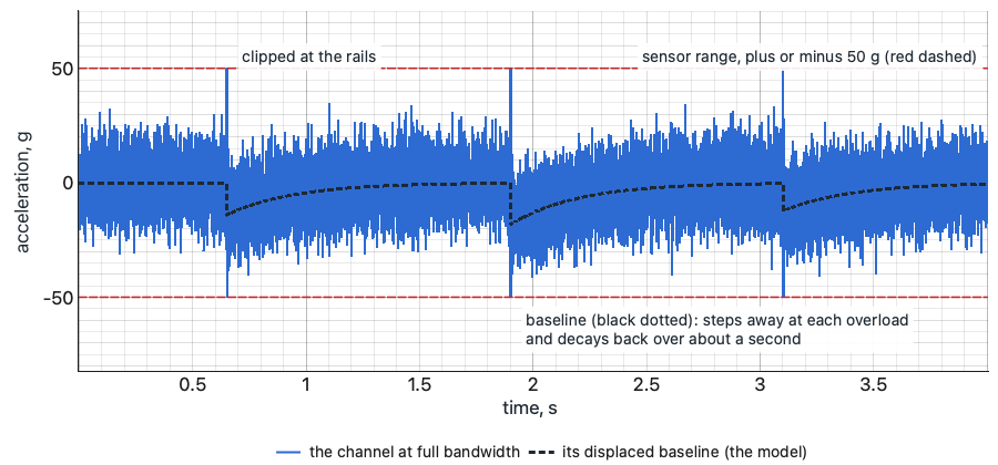
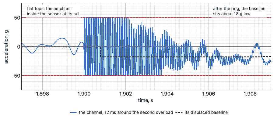
Saturation, and the baseline that decays. When the sensor's built-in amplifier is driven past its range, by a resonance, a random peak, a shock or energy far above the band, it clips, and its output takes time to recover. One sensor manufacturer's note on faults (PCB Piezotronics TN-30) describes the signature: after the overload the baseline of the time history is displaced and decays back exponentially. The same note says such a record can go unnoticed if only frequency-domain data is viewed, and that a low sample rate can mask it. That is the trap. The ASD of a saturated record (the acceleration spectral density, the spectrum a random test is run and judged on, Chapter 7) can look nearly normal, because the decay is slow and sits below the band, the clipped peaks are a small fraction of the record, and the averaging that builds the ASD (Chapter 3) spreads what is left. The check is the time history at full bandwidth, looked at, not the spectrum: flat tops, a baseline that steps and creeps back, peaks against the sensor's range. The cures are a sensor with a higher range, a fix for whatever is rattling, or, for a shock with high-frequency content far above the band, the mechanical filtering Chapter 8 covers.
a. The time history at full bandwidth
Three overloads from a rattle far above the band: spikes to the sensor's 50 g rails, and the baseline stepping away and decaying back.
b. 12 ms around the second overload
Flat tops on both rails while the amplifier inside the sensor is saturated, then the baseline about 18 g low.
c. The ASD of the same record
The saturated record (blue dashed) drawn on the ASD of a clean record of the same motion (thick grey).
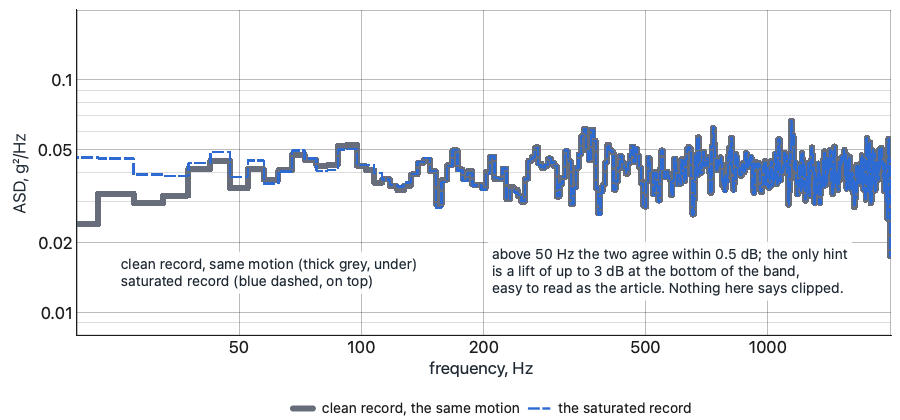
Synthetic record, the author's model of the mechanism: 9 g rms random, 20 to 2,000 Hz; a 100 mV/g sensor with a 50 g range; overloads at 12,000 Hz; recovery time constant 0.3 s.
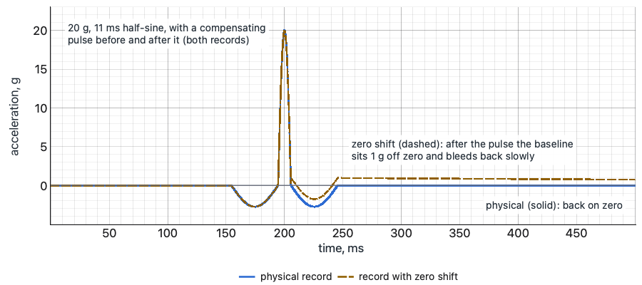
Zero shift on a shock. After a severe shock a piezoelectric sensor can leave an offset in its output that is not motion (1.2). On an AC-coupled chain it shows as a baseline that sits off zero after the pulse and bleeds back at the chain's time constant. Method 516.8, in paragraph 4.4, asks that zero shift be documented and gives the check: integrate the acceleration to velocity. A shaker's table starts a shock at rest and ends it at rest, so the true velocity comes back to about zero after the pulse. A record with zero shift integrates to a velocity that ramps away and keeps going, which no table can do. The check is a few seconds on any analysis package, run on every shock record before the pulse is called good. A channel that fails it is a sensor problem, not a pulse problem, and the cure is the piezoresistive sensor of 1.2.
a. Acceleration
The same shaker shock twice: physical (solid) and with zero shift (dashed).
b. Velocity, the integral
The check: integrate each record to velocity. The physical one returns to zero; the one with zero shift ramps away.
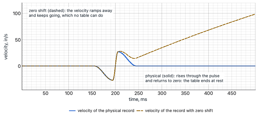
Synthetic: 20 g, 11 ms half-sine with a 2.75 g, 40 ms compensating pulse before and after; zero shift 1 g, bleeding back at a 1 s time constant. Velocity in in/s.
Hum. A comb of narrow, steady peaks at the line frequency and its harmonics, 60 Hz and its multiples or 50 Hz and its multiples, is a ground loop until shown otherwise (1.5). Its signature is that it is there with the drive at zero. The check is a record with the amplifier on and the drive at zero, the noise-floor run of 2.5: the comb that is there is the measurement's, not the article's. Then the loop is broken at the sensor with an isolated mount or at an isolated input, and the record is repeated. If the comb goes, the article was never involved, as the story in 1.5 found.
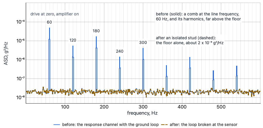
Synthetic: a floor near 2 x 10⁻⁸ g²/Hz; hum at 60 Hz and its harmonics to 540 Hz (50 Hz and its multiples where the line frequency is 50 Hz). 1 Hz lines.
Spikes and dropouts that follow the cable. A spike in the time history that lines up with the cable moving is the cable: triboelectric charge in a charge system (1.5), an intermittent conductor or connector in any system. A dropout, the signal falling to the baseline for a moment and coming back, is a connection opening and closing. Both get worse as the level rises, because the cable moves more. The check is the wiggle test: drive at zero, the channel's time history on the screen, the cable flexed by hand along its run and the connectors pressed and turned one at a time. The spike appears when the fault is touched. The cure is a new cable and the tie-downs that should have held the old one.
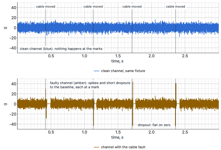
Synthetic: 4 g rms random response, 20 to 2,000 Hz; dotted lines mark when the cable moved. Top: a clean channel beside it. Bottom: the channel with the fault.
A resonance that belongs to the sensor. A peak at the top of the band or above it that is the same on every test, whatever is on the fixture, is the sensor's mounted resonance, excited by whatever the test puts near it. A peak that appears on one channel and not on its neighbors, at a frequency the article's survey never showed, is the sensor's mount. The check is the comparison the opening story missed: the same mode on another channel at the same frequency. A resonance of the structure appears on every channel that sees that mode. One that appears on one channel alone is a sensor until the sensor is cleared, by retorquing, remounting, or moving it to a stud.
A mount coming loose. A mount that is loosening announces itself before it lets go. The high-frequency floor rises, because a loose sensor rattles. Spikes appear at the peaks of the motion, where the sensor lifts and lands. The mount's resonance falls, and a peak walks down the spectrum from one run to the next, as it did in the opening story. And the effect grows with level. The check is a wrench on a stud or a fingernail at the edge of a glue line, between runs, and below the first mode of the fixture and article, the rigid-body check of 4.4: every in-axis channel should read the same there, and a channel that reads differently is the channel, not the structure. A response that changes between the signature runs before and after a full-level run is a finding only after every sensor that shows the change has been checked on its mount.
Drift with temperature. In a chamber, a channel that drifts slowly while the temperature is changing, and settles when it stops, is reading the temperature, not the motion. A compression design responds to a thermal transient in its base (1.2); any sensor's sensitivity follows its temperature curve (1.3). The check is a record with the drive at zero across a temperature change: drift there is the sensor's. The cure is a shear design for the next test and a settled temperature before every run on this one.
Right shape, wrong size. The hardest liars have nothing wrong with their shape. A wrong sensitivity, a gain entered twice, the wrong units or detector, a channel patched to the wrong sensor, a triaxial axis assigned to the wrong channel, a sensor mounted on the wrong axis or upside down: each gives a clean signal of the right form at the wrong level or the wrong sign. 1.1 said why these are invisible on the channel by itself. They are found only by comparison: the calibrator through the chain (1.7), the polarity check of 2.5, the second chain beside the control channel (1.6), and the rigid-body check at the first low level (4.4), where a channel that sits above or below its neighbors below the first mode has no structural excuse.
The order of suspicion is the point of this section. When the data says something strange, the chain is checked before the article is blamed, because the chain's checks take minutes and the article's take days, and because a finding that survives the chain's checks is a finding the analyst can defend. What each check found goes in the log beside the run, because a year later the log is the only place anyone will look (Chapter 14, Chapter 15).
Decide. Every signature in this section has a five-minute check, and the check is run before the article is blamed: the bias, the time history at full bandwidth, the velocity integral of every shock, the record with the drive at zero, the wiggle test, the neighboring channel on the same mode, the wrench on the mount, and the rigid-body check. What the check found, and what was done about it, goes in the log beside the run.
Common Questions
Why can a saturated sensor go unnoticed?
Because the signature is in the time history, not the spectrum (1.8). The baseline's decay sits below the band, the clipped peaks are a small fraction of the record and the averaging spreads the rest, so the ASD can look nearly normal; a low sample rate can mask it too. The check is the time history at full bandwidth: flat tops, and a baseline that steps away and creeps back.
A peak moved after full level on one channel. Is that a finding?
Not yet. A resonance of the structure moves on every channel that sees that mode, so the first check is the other channels on the same mode (1.8). Then the sensor's mount, with a wrench on the stud or a fingernail at the glue line, and the rigid-body check (4.4). A change between signature runs is a finding only after every sensor that shows it has been checked on its mount, the lesson of the chapter's opening.
How can a comb at the line frequency be told from the article's own power supply?
Record with the amplifier on and the drive at zero, then with the article switched off (1.8). A comb that stays with the article off and comes and goes with the amplifier is a ground loop through the cable shields (1.5). Break the loop at the sensor and repeat; if the comb goes, the article was never involved.
Which plot does the operator watch, the time history or the spectrum?
Each catches faults the other hides (1.8). The time history at full bandwidth shows bias, clipping, decay, spikes and dropouts that the spectrum averages away; the spectrum shows hum, resonances and a rising floor that the time history buries. Which one is on the screen while the data comes in is 2.6's subject.
Quiz: Try It
Open book. 5 questions drawn from this section's pool. 4 correct passes the quiz. Nothing is recorded here; in the course your passing attempt opens the next section.